Errata: Elements of 3D Seismology, 2nd edition

Chapter 4


EQ 4.7: plus sign in denominator should be minus sign

Footnote to section 4.3.1: our definition of rho_oil is in disagreement with EQs 18, 19, and 23 of Batzle and Wang (1992). But, in fact, EQ 19 shuld not be used as this would double apply the temperature effect which is accounted for with EQ 23. (M. Batzle, email 2/25/1999).

EQ 4.12: constant 1.115 should be 1.15

Keynote address at Australian SEG

Abstract: In this talk the nature and magnitude of the atmospheric CO2 problem is developed, leading to the push for geologic CO2 sequestration efforts. As an example, our work at the Dickman Field site in Ness County, Kansas is presented. This involves extensive attribute analysis of 3D seismic data, geological property estimation and gridded model-building, followed by flow simulation on regular and refined grids. The goal is to estimate the potential volume of CO2 that could be injected at Dickman as a template for mid-continent sites in the U.S., and quantitative evaluation of the subsurface fate of injected CO2 over long-range simulations lasting several hundred years.

9/11 + 10

On the 10-year anniversary of the World Trade Center attack, it is time to share a note written the morning after.

----------------------------------------------------------

"When you are going through hell, keep going." Winston Churchill

San Antonio (6:30 am, Wednesday, 12 September 2001)

Change
As some readers may know, I have had the honor of serving as SEG Editor for the last two years. With this job go certain responsibilities, time commitments, and priority adjustments. For me, one casualty of this process was the Seismos column which had appeared at erratic intervals since 1992. As my term drew to a close there were requests that I restart Seismos -- they were few, but sincere.

The way it works is this. The new Editor takes over at the close of the annual meeting, which is typically noon Thursday. (So someone with an eye for detail will realize that as I write this I am still Editor for a day-and-a-half.) It seemed natural to mark the end of my term with the (re)beginning of Seismos. I even had a topic. Back in 1992 I wrote a column on ancient Greek seismology, called it Part I, and promised the imminent delivery of Part II, which never came. But now it would, and -- who knows? -- I might win some kind of infamous notoriety for the longest publishing gap in the history of the Society.

To help celebrate all of this I invited my son David (age 16) to San Antonio. He arrived on Monday afternoon and with the help of Larry Rairden and his Porsche 911 we got back to the hotel in time for the Editor's Dinner. At this event the Editor recognizes all those who keep the Society publications going through remarkable volunteer efforts. There were about ninety people in the room and it was a wonderful dinner party; friends, family, laughs and introduction of my successor Gerard Herman. Our scientific and popular press is in very good hands.

It was an early night for me because the nest morning would bring the speaker's breakfast at 7:30, followed by the TLE Forum on Geophysics and the Environment which I was to chair.

David and I scrambled out of bed in time for the breakfast. From there it was a blur of meeting with other session chairmen, final room arrangements and last minute notes. The session began at 8:30 am.

Things went along more or less as expected till about 10 o'clock. The speaker at this point was Dennis Wright, a biologist with Canada Fisheries. At some point I noticed our AV technition, James, had come around behind the speaker's podium to speak with me. In a surreal, slow motion scene I squatted with my ear tilted to hear him over the speaker as he laid out in brief terms the unfolding horror in the world; two hijacked civilian jets, World Trade Center, Pentagon...

I returned to my seat and sat in silence as the speaker continued. A curious mixture of numb shock and darting thoughts washed over me. Then James came again with a printed document and instructions to have me interrupt and read it to the room. With Dennis still at the podium I touched his arm, he stopped, and using the table microphone I read the text from my seat at the table.

"SEG Delegates and Guests: We have a very important announcement...[full text]... and will provide announcements regarding any change in the conference status."

I can make no claim to have handled this well. My voice quavered adn I sat reading while the speaker was stranded at the podium. I offered an open question to the room whether we should proceed or stop the Forum -- someone somewhere nodded and I caught his eye, no one else seemed to move. I took this small affirmation and turned my question to the pane where there was clear spirit to continue. Last (how insensitive can a session chairman be?), I turned to Dennis and asked if he would like to continue. To his great credit, he carried on and finished the talk. Jack Cladwell, our final speaker, did the same. Remarkable people on a remarkable day.

The forum ended, we had lunch on the Riverwalk, then David and I walked evey inch of the exhibition floor. He colleccted every freebie in the place and met dozens of my friends. We did not watch CNN as I resolved early to gt my information in print to filter out the inane real-time speculations.

So my Greek Seismology II Seismos column will have to wait a bit longer. But I will work on it. I will work on it as the world deals with fear and hate and reprisal.

I will work on it while the world changes.

First page of the note hand-written on 9/12/2001.

Phase, phase, phase

My 2002 Seismos column in Leading Edge describing various seismic meanings of the word phase can be found here.

Shane drain

After a 14 hour day at the University of Houston and finishing my 8:30 class last night, I got together with some old Arkansas buddies (Shane, Eddie and John) at the Flying Saucer in downtown Houston.  With four geologists you know the conversation will eventually take a turn toward the oil and gas business.   One recurring theme was the relation of world population and oil production as shown in this plot from another blog entry.

Toward the end of the evening words alone were insufficient to convey the complex ideas springing up. Beer coasters were called to duty as makeshift sketch pads, examples below.

The concept of the Flying Saucer is plates on all walls and ceiling with witty sayings.  My favorite spotted last night: There are three kinds of mathematicians in the world: Those who can count and those who can't. 

A fine session with many of the world's problems solved.  Thanks boys.

*********************************************************

Shane's concept of drainage patterns in a fracked horizontal well over time.

Eddie explains a mysterious horizontal well with a cross section drawing(top) and Shane pushes the drainage pattern theory again (below).

Shane mathematics.

Field Camp Video

I spent a week at the University of Houston Geophysics Field Camp organized by Prof. Rob Stewart.  Here is a short video compiled about the experience.  Enjoy.

Keynote at 2012 ASEG

As part of my 2012 world lecture tour for the SEG DISC, I have been asked to deliver a keynote presentation at the Australian SEG meeting being held 26th – 29th February 2012 in Brisbane, Queensland, Australia.

Title:
Aspects of Reservoir Geophysics for CO2 Sequestration

Abstract:
In this talk the nature and magnitude of the atmospheric CO2 problem is developed, leading to the push for geologic CO2 sequestration efforts. As an example, our work at the Dickman Field site in Ness County, Kansas is presented. This involves extensive attribute analysis of 3D seismic data, geological property estimation and gridded model-building, followed by flow simulation on regular and refined grids. The goal is to estimate the potential volume of CO2 that could be injected at Dickman as a template for mid-continent sites in the U.S., and quantitative evaluation of the subsurface fate of injected CO2 over long-range simulations lasting several hundred years.

Earthquake CDF

This interactive Earthquake document is pretty cool. To view and run it you may need to install the CDF Player (free).

CDF (computational document format) is Wolfram's model for sharing reproducible research documents. In a more general sense, this has been a Jon Claerbout goal for many years. But as you will see from the link, the reproducible research community does not want any commercial software to be involved, only open source tools.

DISC course sequence

2012 SEG Distinguished Instructor Short Course


Elements of Seismic Dispersion: A somewhat practical guide to frequency-dependent phenomena

Christopher L. Liner, University of Houston

Overview

The classical meaning of the word dispersion is frequency-dependent velocity. Here we take a more general definition that includes not just wave speed, but also interference, attenuation, anisotropy, reflection characteristics and other aspects of seismic waves that show frequency-dependence. At first impression the topic seems self-evident: Of course everything is frequency dependent. But much of classical seismology and wave theory is non-dispersive: the theory of P and S waves, Rayleigh waves in a half-space, geometric spreading, reflection and transmission coefficients, head waves, etc. Yet when we look at real data, strong dispersion abounds. This course is a survey of selected frequency-dependent phenomena routinely encountered in reflection seismic data.

1. Time and frequency

The Fourier transform (FT) is a standard frequency analysis tool, but one that yields little information about combined time-frequency content. We will review the FT and its extension to short-time FT and continuous wavelet transform as representative examples of a broad class of time-frequency decomposition methods.

2. Vibroseis harmonics

The vibroseis source injects a long, slowly varying signal into the earth. We commonly find that new frequencies, or harmonics, not present in the sweep are present in the earth response. This interesting phenomena is discussed in relation to a more familiar process, that of human hearing. These harmonics are illustrative of a general property of nonlinear waves and interaction.

3. Near surface

Velocity dispersion is generally considered not to be an issue in seismic data processing. But that is a sloppy compression of reality. It is pretty nearly true for seismic body waves (P, S, and mode converted) moving around the far subsurface. In the near surface, however, velocities often show strong dispersion and the description is terribly inaccurate. This is especially the case in marine shooting over shallow water where, even in the 10-100 Hz band, velocities are observed well above and blow the speed of sound in water. This paradox arises because shallow water over an elastic earth forms a waveguide whose characteristics we will examine.

4. Anisotropy

This chapter deals with seismic velocity anisotropy and how it depends on frequency. We will restrict our comments here to velocity variation with respect to the vertical axis (VTI) in a horizontally layered earth. Of the sedimentary rock types, only shale is seen to be significantly anisotropic at the core, or intrinsic, scale. The question is how to calculate apparent anisotropic parameters of a layered medium as seen by very long waves. Backus (1962) solved this problem and his method can be applied to standard full wave sonic data. So where does dispersion come into all this? It is buried in the thorny question of the Backus averaging length.

5. Attenuation

The distinction between intrinsic and apparent frequency-dependent seismic properties is nowhere greater than in the area of attenuation. In this chapter constant Q and viscous theories of intrinsic attenuation are developed and compared to experimental intrinsic scattering attenuation data. Intrinsic attenuation is found to be compatible with the viscous theory, while constant Q yields a better explanation of scattering attenuation due to layering.

6. Interference

The preceding chapters have explored frequency-dependent phenomena related to acquisition and wave propagation, effects that would be seen and dealt with on prestack data. Data processing will remove or correct for these effects and be unseen by the interpreter. But dispersion effects (in our broad meaning) remain in the realm of final imaged data. First and foremost is the fundamental, unavoidable phenomena of interference. We will discuss selected topics in this broad field, including the thin bed, bandwidth effect on reflectivity, single frequency isolation, and reflection from a vertical transition zone.


7. Biot reflection

Many of the dispersion effects discussed previously contain information about the subsurface, but none as direct and important as the problem of reflectivity dispersion due to a poroelastic contact in the earth. We will review the nature of body waves in porous media, the characteristics of Biot reflection from an isolated interface, and wrap up with an introduction to Biot reflections in layered porous media.

Learning Goals

• Gain a broad understanding of dispersive phenomena and related investigation tools.
• Understand the fundamental difference between intrinsic and apparent dispersion phenomena.
• Improve knowledge of the reflection process beyond the classic model.
• Provide an appreciation of historical development and a deep guide to the literature for self-study.

Who Should Attend

The course is framed along the lines of acquisition, processing and interpretation to, hopefully, contain material of interest to the entire spectrum of seismic geophysicists. The mathematical level of the course is generally on the advanced undergraduate level, but deeper aspects are often included for advanced readers. Familiarity with the Fourier transform and related topics would be beneficial. In all cases, theoretical developments are illustrated by examples or case histories.

Biography


Christopher L. Liner joined the faculty of the University of Houston Department of Earth and Atmospheric Sciences in January 2008 and is now professor and associate director of the Allied Geophysical Laboratories industrial consortium. He earned a bachelor of science degree in geology from the Univer- sity of Arkansas in 1978, a master of science in geophysics from the University of Tulsa in 1980, and a Ph.D. in geophysics from the Center for Wave Phenomena at Colorado School of Mines in 1989. He began his career with Western Geophysical in London as a research geophysicist, followed by six years with Conoco. After working a year with Golden Geophysical, he served as a faculty member of the University of Tulsa Department of Geosciences from 1990 to 2004. From 2005 through 2007, Liner worked as research geophysicist with Saudi EXPEC Advanced Research Center, Dhahran, Saudi Arabia.

Liner’s research interests include petroleum reservoir characterization and monitor- ing, CO2-sequestration geophysics, advanced seismic-interpretation methods, seismic data analysis and processing, near surface, anisotropy, and seismic wave propagation. He served as editor of GEOPHYSICS in 1999–2001 and contributing editor to World Oil in 2010 and is an editorial board member for the Journal of Seismic Exploration. Liner has written many technical papers, abstracts for scientific meetings, the “Seismos” column in THE LEADING EDGE (since 1992), the “Seismos Blog,” and the textbook Elements of 3D Seismol- ogy, now in its second edition. Liner is a member of SEG, AAPG, AGU, the Seismological Society of America, and the European Academy of Sciences. In 2011, he was named an honorary member of the Geophysical Society of Houston.

Nonlinear wave propagation

Just a comment about harmonics and nonlinear waves. Whatever their physical origin in the machinery, vibroseis harmonics can be considered as generated by asymetric (nonlinear) up and down motion of the baseplate interacting with the earth. I have written about this elsewhere. We can say this is nonlinear interaction between the machine and the earth, although linear wave propagation occurs in the air and earth near surface. This kind of nonlinearity is interesting and common, but there is an other kind of much greater interest.

When wave equations are nonlinear, then we say the medium is nonlinear. New kinds of phenomena emerge not present in linear wave propagation. For example, when two linear waves meet the amplitude is the sum of the two waves. Not so with nonlinear waves. The primary feature of a nonlinear wave is that it's velocity depends on the peak amplitude. Linear wave velocity does not depend on peak amplitude. There are many examples, a classic being the Korteweg & de Vries equation describing solitons (non-dissapating waves) in a narrow water channel.

Why is all of this nonlinear stuff is of interest to geophysicists? Because the theory of poroelasticity (as developed originally by M. A. Biot in the 1950s) leads to wave equations that are nonlinear. when such a medium is probed by a harmonic signal (single frequency), asymmetries will develop in the propagated wave. The response will repeat the same number of times per second as the input, but because it is no longer a perfect sine or cosine a Fourier transform will reveal the original frequency and a series of harmonics. Encoded in the spacing and amplitude of the harmonics is key information about the medium, such a fluid viscosity and permeability. But it is an open question how to do in situ experiments to reveal this phenomena and, if we could, it is not known how to unravel the important information contained therein.

P.S. Steven Wolfram has written a fascinating interactive nonlinear wave equation explorer. A couple of plots are given below.

Linear waves interact by superposition just as we think they should.

Interaction of nonlinear waves is much more complicated and the details depend on the nature of the wave equation.

Agile* cheatsheets and more

Agile* is a fascinating and very modern blog that includes free geophysical phone apps for Android and very cool summary posters on geophysical topics (cheatsheets).

At the time of this blog entry cheatsheerts include Basic, Geophysics, Rock Physics, and Elastic Properties From Sonic Logs. These have to be seen to be believed, here is the Geophysics one as a tease to the rest:

I am sure the list will change over time, so you may want to checkout the Agile* download area once in a while.

Also very thoughtful is the scales of geoscience diagram:

The minds behind Agile* are Matt Hall and Evan Bianco. Great work!! In my opinion, they are the next stage of evolution in communication, organization, and sharing of geoscience knowledge.

Greek to Greek

Dear Panagiotis,

How appropriate that my book Greek Seismology should be translated into Greek by your students. You have my permission to publish the translation. Please send me the link when the book is published online. 

Best regards,

Prof. Christopher L. Liner
Dept. of Earth and Atmospheric Sciences
University of Houston

***********************
On May 29, 2011, at 9:47 AM, pantou@pantou.gr wrote:

Dear Sir,

My name is Panagiotis Toumpaniaris, I teach physics and I am coordinator of an environmental group of pupils(ages14-15) of the  Experimental Gymnasium of Iraklion (Πεοραματικό Γυμνάσιο Ηρακλείου).

We are very happy to have found in the internet your work about Greek Seismology. We must say that we found your work excellent and we decided to translate it in Greek! We managed to translate the whole book and we would like to ask your permission to publish our work without any financial profit for us of course! This means that the translatiοn will appear in the site of our school and also in a cd handed out to the office of environmental education.
 
Sincerely
 
Panagiotis Toumpaniaris
Physics Teacher at  the Experimental Gymnasium of Iraklion
Diplom Meteorologe

Rayleigh wave dispersion and shear wave speed

Sensitivity of Rayleigh wave dispersion to shear wave speed for a model consisting of one layer over an infinite half-space. Synthetic shot records (not shown) were generated by Tong Fei's elastic 2D modeling code (sufctanismod.c) and dispersion curves computed using Park's method as implemented by C. Liner (suphasevel.c). Both codes are distributed with the Seismic Un*x free processing system).

AGL meeting 2011

Allied Geophysical Lab tour during our 2011 sponsor meeting (29 April). I am wearing a tie and illustrating something with my fists. Can you find the famous geophysicists? (Leon Thomsen, Brian Russel, and Jim Gaiser). Photo credit: Larry Rairden (EOS Energy)

Fig: Peak amplitude and Q

Figure 1. Theory

Figure 2: Field data

Kurdish oil seep (update)

Back in a Jan 2011 blog entry I showed a great oil seep outcrop photo and referred there to the Atrush-1 well then being drilled nearby. It was recently announced the well came in with initial production potential (IP) of about 6400 barrels per day of 26.5 gravity oil.

Also of note, it looks like an oil export agreement might be back in place to actually allow oil production from the Kurdistan region of Iraq. Squabbling between the Kurdish regional government and the central government in Bagdad had stopped exports for a while, the main hang-ups being revenue sharing and which government entity gets the initial money and makes the split.

Fig: Spectral notches

As I continue to wrap up the SEG DISC book, I will be posting figures once in a while that I think are particularly interesting. No comment, just the figure.

Spectral decomposition at Dickman (3)

(Tim Brown and C. Liner)

See also: Spectral decomposition at Dickman (2)

In an ongoing effort to effectively identify geological features within our seismic volume it is important to have reliable filtering capabilities. Filtering techniques have been applied to our seismic volume using both Seismic MicroTechnology (SMT) and Seismic Unix (SU) to aid in identifying geological anomalies. However, significant differences arise when attempting to use narrow band-pass filters within SMT, especially at low frequencies.

After applying a trapezoidal filter centered on 5 Hz (Figure 1 lower left), it is clear that residual frequencies still reside in the data. The frequency spectrum of the 5 Hz data supports this observation (Figure 1 lower right).

Figure 1. Arbitrary section in Dickman 3D after SMT 5 Hz trapezoidal filter (inset lower left), notice higher frequencies still remain in the data as evidenced by the spectrum (inset lower right).

Application of a similar isolation filter in SU yields something closer to a pure 5 Hz decomposition. This 5 Hz attribute was imported into SMT and the results are displayed in Figure 2. The seismic section shows a low-frequency character expected of a 5 Hz decomposition, and this is supported by its associated frequency spectrum (Figure 2 lower right).

Figure 2. Arbitrary section in Dickman 3D data after SU 5 Hz narrow-band filter.

We compare the results from the two filtered outputs to emphasize these are not esoteric differences. Figure 3 shows an 848 ms time-slice from the SU 5 Hz data, clearly indicating linear features present in the center portion of the survey area. However, these linear features are absent in the SMT 5 Hz time-slice (Figure 4). This discrepancy between the two data sets is problematic because using narrow-band filters at low frequencies in SMT becomes an unreliable method to enhance these important features that may be related to fracturing. In our case, it is important to have a functioning isolation filter because the linear features are only evident at these lower frequencies when using spectral decomposition.

Figure 4. Timeslice at 848 ms in SU 5 Hz data showing diagonal features parallel to the yellow dash line. These are being investigated as a possible fracture indicator.

Figure 5. Timeslice at 848 ms in SMT 5 Hz data without diagonal features. Yellow line as in Figure 4 for reference.

The Curious Case of US Oil Production

I have lately been updating my oil production numbers and plots, first Oklahoma, Texas, and world (OTW) production then Saudi Arabia. In the OTW blog entry I mentioned that I was still working on a US production update.

Digging through my thousands of files, I was able to relocate the data for US oil production from 1857 to 2006. This data had been carefully constructed from various sources and I wrote a Leading Edge Seismos column using it in May 2008. Here is the daily production figure from that column:

Figure 1. Daily US oil production plot from 2008 Seismos column.

Since I finally found the data behind the plot, it seemed a simple matter to add the last 4 years of production  and format the plot like the others I had posted in this blog. 

Naturally, the first place to turn in such matters is the venerable BP Statistical Review.  But something was immediately confusing to me.  Note my data in Fig 1 shows annual production for the US (including offshore and Alaska) as 5.14 MMBO/D. The BP Review showed 6.84 million BO/D for the same year, a whopping 33% difference. Confused, I then checked the Energy Information Administration and found values similar to BP. 

Was I going crazy? I'm not getting any younger, you know. Maybe this was a case of some mild stroke that left me in a confused world. But no, the Seismos column was there as evidence. So maybe I just used bad data back then. But no, wikipedia shows the same thing, and I read a recent paper (Nashawi et al., 2010) containing a daily US production plot (fig 15) that syncs perfectly with mine. Here it is:

Figure 2. US production from Nashawi et al. (2010)

Well, research is what I do, so the chase was on. The result is summarized in Fig 3.  The data comes from my earlier research (green dots), BP Statistical Review 2010 (BP, red dots), the Energy Information Administration (EIA, blue dots), and one data point each from International Energy Agency (IEA, white triangle),  and American Petroleum Institute (API, white square).  The IEA number (244840  thousand tonnes per day) needs a bit of conversion.  Wolfram|Alpha shows this represents 1.68 x 10^9 barrels of oil, or 4.603 million barrels per day.  


Clearly, I would be curious to see a full series of production numbers from IEA or API, but have been unable to figure out if these groups keep historical data on the internet.  

Figure 3. The mystery in a nutshell.  My green trend is supported by 2008 and 2010 numbers from API and IEA.  Meanwhile, BP and EIA are about 30% higher.  What the heck is going on?

Figure 4. Detail of Fig 3 from 1960-2010

At this point I have no resolution to the mystery, I just wanted to lay it out for all to see.  It is hard to imagine this discrepancy is due to definitions of crude oil (e.g, is shale oil included? condensate? heavy oil?).  Any of these would be in the accounting noise, not a 30% difference.


Comments are welcome.

References:


Liner, C., 2008, To peak or not to peak, The Leading Edge 27, 610.

Nashawi, I.S., Malallah, A., and Al-Bisharah, M., 2010,Forecasting World Crude Oil Production Using Multicyclic Hubbert Model, Energy Fuels, 24, 1788-1800.

Note: Along these same lines, North Dakota is producing more oil than ever.

What is the SEG DISC?

As mentioned before in this blog (here, and here), I have been honored by selection as the 2012 SOciety of Exploration Geophysicists DISC presenter. My department chairman wanted a newsletter blurb. Here goes...

What is the DISC?

The SEG Distinguished Instructor Short Course (DISC) is an eight-hour, one-day short course on a topic of current and wide-spread interest. Sponsored by the SEG, it is presented at 30 locations around the world. Established in 1998, the DISC has attracted over 25,000 participants in its 14-year history.

Selection as the DISC instructor is viewed as a major honor and recognition of excellence by the SEG. The instructor is a prominent geophysicist whose work and presentation appeal to a wide audience ranging from students to mature professionals.

The DISC is recorded each year and developed into a multimedia presentation called the DigitalDISC, which features the video of the instructor, transcript of the lecture, and presentation slides. This DigitalDISC is distributed as a service to student sections, and is available for purchase from the SEG Book Mart.

The 2012 DISC, presented by Christopher Liner, is on the topic of Seismic Dispersion. Toward the end of 2012, it will be available in ebook form or print edition.

10000 Visitors

Today the Seismos blog passed ten thousand visitors, a mere 1 year and 17 days after passing the one thousand mark.  That is a ten-fold increase in just about a year and the trend is accelerating, as can be seen in the plot below.  This was generated in Excel using data from the StatCounter I have on the blog.

The blog started 4 October 2008, but the stat counter only has data from 1 Sept 2009.

I have added a trend line to the Page Loads curve and the best fit I could get was using a 4th order polynomial (see equation). Extrapolating this trend predicts the 20k mark will be reached about 670 days after 1 Sept 2009 which works out to be 3 July 2011. The next 10-fold increase to 100k should be in Feb or March 2012.

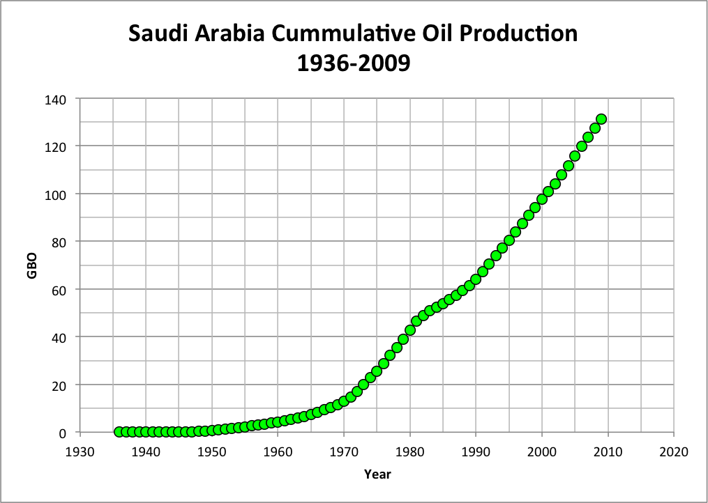
Saudi Arabia Oil Production Update: 2009

Following an earlier post with updated Oklahoma, Texas, and world oil production plots, I was motivated to review and revise my Saudi Arabia production numbers.  KSA (Kingdom of Saudi Arabia) production began in 1936 and my plots start there, but I am unable to identify the source of my early numbers (1936-1964).  Nothing sinister, my computer files are growing at about 38GB/yr and I can't find the original data source.  For 1965-2009 I use the BP statistical review.

I must admit this was somewhat motivated by this recent story.  I have done my own estimates and may report that sometime.

For now, let's stick to the production data.  I was in KSA from 2005 through 2007 and note those years included the daily production peak (so far) and two years of decline.  As soon as I left, production went up.  Fascinating.

Dickman Project Overview

The goals of this DOE-funded project were to develop innovative 3D seismic attribute technologies and workflows to assess the structural integrity and heterogeneity of subsurface reservoirs with potential for CO2 sequestration. Our specific objectives were to apply advanced seismic attributes to aide in quantifying reservoir properies and lateral continuity of CO2 sequestration targets.

Our study area (Figure 1) is the Dickman field in Ness County, Kansas, a type locality for the geology that will be encountered for CO2 sequestration projects from northern Oklahoma across the U.S. mid-continent. Since its discovery in 1962, the Dickman Field has produced about 1.7 million barrels of oil from porous Mississippian carbonates (Figures 2 and 3) and basal Pennsylvanian sandstone (Figure 4) that locally develops on a regional MIss-Penn unconformity surface. The Dickman field includes a small structural closure at about 4400 ft drilling depth. Project data includes 3.3 square miles of 3D seismic data, 142 wells, with log, some core, and oil/water production data available. Only two wells penetrate the deep saline aquifer. Geological and seismic data were integrated to create a geological property model and a flow simulation grid.

We systematically tested over a dozen seismic attributes, finding that curvature, SPICE, and ANT were particularly useful for mapping discontinuities in the data that likely indicated fracture trends. Recently we have been studying spectral decomposition as a way to detect additional channel details and fracture trends.

Our simulation results in the deep saline aquifer indicate two effective ways of reducing free CO2: a) injecting CO2 with brine water, and b) horizontal well injection. A tuned combination of these methods can reduce the amount of free CO2 in the aquifer from over 50% to less than 10%.

Figure 1. Dickman field site and description of available data.

Figure 2. Annotated type log for Dickman project area (black circle in Fig. 1).

Figure 3. Chart to the left is the stratigraphic rank accepted by the Kansas Geological Survey (Sawin et al., 2008). The chart to the right shows correlation to Dickman local stratigraphic units, with higher confidence correlations in bold. The blue vertical bar indicates the target strata for Dickman research.

Figure 4. Time slice through 3D amplitude volume at 850 ms (approximate top Miss level) showing clear evidence of incised channel. Geological interpretation along highlighted line on right.

Spectral decomposition at Dickman (2)

(C. Liner and J. Seales)

In and earlier post, spectral decomposition (SD) of the the Dickman 3D data using simple bandpass filtering. This has been done using both seismic unix and SMT filtering tools. Here we consider the sensitivity of the SD output on choices of the filter parameters.

A broadband time slice (847 ms) through the data shows a well-defined channel. Aside from a slight amplitude change to the SW, we see no evidence of overbank or secondary channel features.

Figure 2 is an SU plot created using a filter centered on 41 Hz generated by a shell script. The image shows a clear feature that trends away from the channel to the SW. The filter parameters are shown along with a dash-yellow outline of the feature under discussion.

Equivalent 41 Hz time slices at 847 ms (Figures 3 and 4) were created using the trapezoid filter in SMT. Apart from grayscale color bar differences between SU and SMT, the time slice features are consistent between SU and SMT. Both filters created in SMT were centered on 41 Hz, but Figure 3 uses a 2 Hz top while Figure 4 is more constrained with a 0.2 Hz top. Visually, these results are equivalent indicating the SD attribute computed in this manner is not unstable with respect to filter parameter choices.

To study detailed variation between these SMT results, subtractive difference volumes were generated using functionality in SMT (Figures 5 and 6). These show there are, indeed, slight differences between the output of the two SMT filters created. Both figures show the same result, but with opposite amplitudes due to changing the subtraction order. The difference plots show energy in horizontal bands representing acquisition footprint (source orientation), a large fault in the NW corner, a bright karst (sinkhole) feature near the center, and a network of curved lineations of unknown origin. In an absolute sense, the maximum amplitude difference between the 2Hztop and 0.2Hztop filters is on the order of 10% in the mentioned features, otherwise it is less that 2%.

If this kind of spectral decomposition is to be generally useful, it is important to quantify the sensitivity on filter parameters beyond the visual difference described above. To accomplish this, we set out a grid of 27 points in the 3D survey area about 2500 ft apart (Figure 7). At each location, the amplitude for 2Hztop and 0.2Hztop results were measured and cross plotted in Excel (Figure 8).

Figure 7. Test point grid for amplitude cross plot between the SMT filter results.

Figure 8. Amplitude cross plot between selected locations in the two SMT filter spectral decomposition results (diagonal line would be exact equality). No significant differences are indicated,

Finally, we notice that an 847 time slice through the SPICE attribute volume (Figure 9) seems to indicate the same channel feature seen on 41 Hz spectral decomposition results. We are planning further investigation of this tantalizing relationship.

Figure 9. SPICE attribute time slice at 847 ms showing feature similar to the 41 Hz channel feature.

Madagascar on Mac OS X

I am experimenting with Madagascar, a public domain processing system descended from SEPlib. My plan is to use seismic unix (SU) as usual for graphics and most analysis, but M brings some important new functionality that is not in SU. Specifically, more 3D applications and parallel computing capability (my power mac has 8 cores, a mini cluster).

Here is an outline of how to install Madagascar on Mac OS X. This worked on my powerbook and desktop power mac. The workflow assumes you have already installed the Xcode development tools and gfortran or g95.

(1) Download Madagascar source from sourceforge:

http://sourceforge.net/projects/rsf/files/

(2) In your downloads folder, double click on the zip file to unpack. A new folder will be created named madagascar-1.1 with all the stuff in it.

(3) Make a directory ~/usr/local (~ means your home directory)

(4) Move the folder from item (2) to ~/usr/local

(5) Install Java for Mac OS X 10.6 Update 3 Developer Package. You must have a mac developer account.

(6) As superuser, use macports to install scons. Note: this will fail while installing db46 unless you have done step (5).

(7) In the directory ~/usr/local/madagascar-1.1 type configure at the command line. This will create a file named env.csh

(8) Assuming you are using the tcsh shell, you will have a file in your home directory named .tcshrc which is a resource file for tcsh. It is invisible to the finder (due to the leading dot), but can be seen and edited using the vi editor. Open the env.csh file and copy its contents (except the leading line) to the bottom of your .tcshrc file. Close the file and quit/restart the terminal application.

(9) As superuser in ~/usr/local/madagascar-1.1 type make and when that completes type make install

(10) Exit superuser and type rehash

(11) If all goes well, you can proceed to test your install as described on this page

Here is a simple test that worked (thanks to some advice from Sergy Fomel):

================ makefile ================

================ terminal output ================

================ Graphics result ================

Spectral decomposition at Dickman

In our ongoing effort to relate seismic attributes to geologic features at Dickman, we have generated a series of narrow-band attribute volumes from the migrated data. Unlike traditional time-frequency methods (Chakraborty and Okaya, 1994) that seek a trade-off of time and frequency resolution, we have chosen to use a pure frequency isolation algorithm. In fact, the method we use is traditional Fourier bandpass filtering with a very narrow response centered on the frequency of interest. In Figure 1 we show (a) the original 3D migrated data spectrum as extracted in a 5x5 bin area, (b) the same after narrow band filtering around 6 Hz and (c) after 43 Hz narrow band filtering.

Figure 1. Spectrum of Dickman seismic data and narrow band decomposition. (a) Fourier amplitude spectrum of 3D migrated data in a 5x5 bin area from 0-2 seconds. (b) Spectrum after narrow bandpass filtering centered on 6 Hz. (c) Spectrum after 43 Hz narrow bandpass filtering.

In the vertical view (Figure 2) the narrow band results are not very enlightening. It is tempting to conclude the new data has no time information content, but in fact there is time localization in the amplitude modulation of each trace although it seems to have little value in the vertical view.

Figure 2. Representative seismic line before and after filtering. (a) Original broadband data. (b) Narrow band 6 Hz data. (c) Narrow band 43 Hz data.

Figure 3 shows a time slice through the broadband data at 848 ms, roughly coincident with the Miss/Penn unconformity. The prominent incised channel is clearly shown. Note there are no clear trends in the data aligned with the yellow dash lines and the channel does not seem to approach the tip of the yellow arrow.

Figure 3. Broadband timeslice at 848 ms, approximately coincident with the Miss/Penn unconformity. Features observed in narrow band data (Figs 12 and 13) but not on the broadband data are indicated in yellow.

A coincident time slice through the 6 Hz data (Figure 4) shows a strong and remarkable diagonal alignment parallel to the yellow dash lines. One always suspects acquisition footprint when linear features show up in seismic data, so Figure 5 shows the shot and receiver orientation for the Dickman 3D data. While it is possible the NW-SE trend is related to source line orientation, the conjugate direction has no association with shooting geometry. We suspect these features indicate fracture orientation as described using curvature by Nissen et al. (2004, 2006). We plan to investigate this alignment further in the next quarter.

Figure 4. Narrow band (6 Hz) timeslice at 848 ms. Yellow dash lines indicate orientation of diagonal features (perhaps related to fractures) not seen in Fig 3.

Figure 5. Shooting geometry orientation for Dickman 3D, shots (L) and receivers (R).


At a higher frequency band (43 H, Figure 6) we observe a dark channel-like feature as indicated at the tip of the yellow arrow. We are currently working to confirm or deny the reality of this channel feature. The process will consist of studying well logs inside and outside the feature; particularly concentrating on basal Pennsylvanian sediments and indications of a subtle structural low at the top Mississippian.

Figure 6. Narrow band (43 Hz) timeslice at 848 ms. Yellow arrow indicates channel feature not seen in Figure 3.

Method

Spectral decomposition (SD) figures shown above were generated using SeismicUnix (SU) on segy data output from SMT's Kingdom software. Specifically the sufilter program was driven by a shell script that implemented the following steps:

for each frequency of interest, stepping by 1 Hz {
__read segy and convert to SU format
__set params to isolate one frequency
__apply sufilter
__extract time slice
__create pdf figure
}

This allowed quick narrow band data scanning for features of interest in a common time slice. Once a particular narrow band was selected for further analysis, sufilter was applied to the original data and the entire SD attribute volume was output in segy format. This was imported to SMT for further analysis.

While the multiple-frequency scanning cannot be currently done in SMT, a narrow band SD of the type described here can be calculated (Figures 8 and 9) using Tools>>Trace_Pak...>>Process_Multiple_Traces....

Figure 8. Parameter window to create narrow band data directly in SMT Kingdom using TracePak, generating a new data type named amp_6Hz_SMT.

Figure 8. Narrow band (6 Hz) time slice generated and displayed in SMT Kingdom. Compare Figure 4 showing 6 Hz data generated and displayed using SeismicUnix.

Similarity of the SU and SMT result is reassuring, suggesting the linear features are robust features of the data and not merely artifacts related to a particular implementation of bandpass filtering.

References

Nissen, S. E.,T. R. Carr, and K. J. Marfurt, 2006, Using New 3-D Seismic attributes to identify subtle fracture trends in Mid-Continent Mississippian carbonate reservoirs: Dickman Field, Kansas, Search and Discovery, Article #40189.

Nissen, S. E., K. J. Marfurt, and T. R. Carr, 2004, Identifying Subtle Fracture Trends in the Mississippian Saline Aquifer Unit Using New 3-D Seismic Attributes: Kansas Geological Survey, Open-file Report 2004-56.